The Ultimate Playlist - Hustle & Heart 🎶

Author

Dhruv

Published

April 25, 2025

🎧 Introduction

From millions of Spotify tracks and playlists, Hustle & Heart emerges as a curated sound journey built on energy, emotion, and authenticity. This project explores what makes songs stick — analyzing popularity, danceability, and musical DNA — before distilling it all into a final 12-track playlist that hits with both data and vibe.

🎶 Just here for the playlist? Tap here

⚙️ Setup: Load & Install Required Packages

This chunk ensures all necessary R packages are installed and loaded before running the rest of the analysis. ✅📦

Code

ensure_package <- function(pkg){
  if (!requireNamespace(pkg, quietly = TRUE)) {
    install.packages(pkg, repos = "https://cloud.r-project.org")
  }
  library(pkg, character.only = TRUE)
}

required_packages <- c(
  "dplyr", "stringr", "tidyr", "purrr", "readr", "jsonlite",
  "ggplot2", "scales", "DT", "rvest", "httr2", "tibble"
)

invisible(lapply(required_packages, ensure_package))

options(dplyr.summarise.inform = FALSE)

🎧 Spotify Style Setup

This chunk sets a custom Spotify-themed style for all plots and tables to give the report a bold, immersive aesthetic. 🎨🟢🖤

Code

library(ggplot2)
library(kableExtra)

theme_spotify <- function() {
  theme_minimal(base_family = "Arial") +
    theme(
      plot.background = element_rect(fill = "#191414", color = NA),
      panel.background = element_rect(fill = "#191414", color = NA),
      panel.grid = element_line(color = "#1DB954", linewidth = 0.1),
      text = element_text(color = "white"),
      axis.title = element_text(face = "bold", color = "white"),
      axis.text = element_text(color = "#b3b3b3"),
      plot.title = element_text(size = 16, face = "bold", color = "#1DB954"),
      plot.subtitle = element_text(size = 12, color = "#b3b3b3")
    )
}

spotify_table <- function(df, caption_text = "") {
  knitr::kable(df, format = "html", caption = caption_text) |>
    kableExtra::kable_styling(
      full_width = TRUE,
      bootstrap_options = c("striped", "hover", "condensed", "responsive"),
      position = "left"
    ) |>
    kableExtra::row_spec(0, background = "#1DB954", color = "white") |>
    kableExtra::kable_styling(font_size = 14)
}

🎧 Task 1: Load Spotify Song Characteristics

In this first task, we download and clean a Spotify song characteristics dataset made available via GitHub. The dataset includes song-level features such as danceability, energy, valence, and more. Our goal is to create a clean, rectangular dataset where each row corresponds to a single artist-song pair.

id	name	duration_ms	release_date	year	acousticness	danceability	energy	instrumentalness	liveness	loudness	speechiness	tempo	valence	mode	key	popularity	artist
6KbQ3uYMLKb5jDxLF7wYDD	Singende Bataillone 1. Teil	158648	1928	1928	0.995	0.708	0.1950	0.563	0.1510	-12.428	0.0506	118.469	0.7790	1	10	0	Carl Woitschach
6KuQTIu1KoTTkLXKrwlLPV	Fantasiestücke, Op. 111: Più tosto lento	282133	1928	1928	0.994	0.379	0.0135	0.901	0.0763	-28.454	0.0462	83.972	0.0767	1	8	0	Robert Schumann
6KuQTIu1KoTTkLXKrwlLPV	Fantasiestücke, Op. 111: Più tosto lento	282133	1928	1928	0.994	0.379	0.0135	0.901	0.0763	-28.454	0.0462	83.972	0.0767	1	8	0	Vladimir Horowitz
6L63VW0PibdM1HDSBoqnoM	Chapter 1.18 - Zamek kaniowski	104300	1928	1928	0.604	0.749	0.2200	0.000	0.1190	-19.924	0.9290	107.177	0.8800	0	5	0	Seweryn Goszczyński
6M94FkXd15sOAOQYRnWPN8	Bebamos Juntos - Instrumental (Remasterizado)	180760	9/25/28	1928	0.995	0.781	0.1300	0.887	0.1110	-14.734	0.0926	108.003	0.7200	0	1	0	Francisco Canaro
6N6tiFZ9vLTSOIxkj8qKrd	Polonaise-Fantaisie in A-Flat Major, Op. 61	687733	1928	1928	0.990	0.210	0.2040	0.908	0.0980	-16.829	0.0424	62.149	0.0693	1	11	1	Frédéric Chopin
6N6tiFZ9vLTSOIxkj8qKrd	Polonaise-Fantaisie in A-Flat Major, Op. 61	687733	1928	1928	0.990	0.210	0.2040	0.908	0.0980	-16.829	0.0424	62.149	0.0693	1	11	1	Vladimir Horowitz
6NxAf7M8DNHOBTmEd3JSO5	Scherzo a capriccio: Presto	352600	1928	1928	0.995	0.424	0.1200	0.911	0.0915	-19.242	0.0593	63.521	0.2660	0	6	0	Felix Mendelssohn
6NxAf7M8DNHOBTmEd3JSO5	Scherzo a capriccio: Presto	352600	1928	1928	0.995	0.424	0.1200	0.911	0.0915	-19.242	0.0593	63.521	0.2660	0	6	0	Vladimir Horowitz
6O0puPuyrxPjDTHDUgsWI7	Valse oubliée No. 1 in F-Sharp Major, S. 215/1	136627	1928	1928	0.956	0.444	0.1970	0.435	0.0744	-17.226	0.0400	80.495	0.3050	1	11	0	Franz Liszt

Task 2: Import Playlist Dataset

We responsibly download and combine all JSON playlist slices into a single list for future processing.

Code

load_playlists <- function() {
  library(jsonlite)
  library(purrr)
  
  dir_path <- "data/mp03/data1"
  if (!dir.exists(dir_path)) dir.create(dir_path, recursive = TRUE)
  
  base_url <- "https://raw.githubusercontent.com/DevinOgrady/spotify_million_playlist_dataset/main/data1/"
  starts <- seq(0, 999000, by = 1000)
  file_names <- sprintf("mpd.slice.%d-%d.json", starts, starts + 999)
  file_paths <- file.path(dir_path, file_names)
  
  for (i in seq_along(file_names)) {
    if (!file.exists(file_paths[i])) {
      url <- paste0(base_url, file_names[i])
      tryCatch({
        download.file(url, destfile = file_paths[i], mode = "wb", timeout = 300)
      }, error = function(e) {
        message("⚠️ Failed to download: ", file_names[i])
      })
    }
  }

  read_playlist_file <- function(path) {
    tryCatch(
      fromJSON(path)$playlists,
      error = function(e) {
        message("❌ Skipping corrupted file: ", path)
        return(NULL)
      }
    )
  }

  valid_paths <- file_paths[file.exists(file_paths)]
  playlists_list <- map(valid_paths, read_playlist_file)
  playlists_list <- compact(playlists_list)
  
  return(playlists_list)
}

PLAYLISTS_LIST <- load_playlists()
all_playlists <- PLAYLISTS_LIST %>% list_rbind()
DT::datatable(
  head(all_playlists, 10),
  options = list(
    pageLength = 6,
    dom = 'tip',
    scrollX = TRUE
  ),
  class = "display compact stripe hover",
  rownames = FALSE
)

🎼 Task 3: Rectify Playlist Data to Track-Level Format

We flatten the hierarchical playlist JSONs into a clean, rectangular track-level format, stripping unnecessary prefixes and standardizing column names.

Code

strip_spotify_prefix <- function(x){
  str_extract(x, ".*:.*:(.*)")
}

rectified_data <- all_playlists %>%
  select(
    playlist_name = name,
    playlist_id = pid,
    playlist_followers = num_followers,
    tracks
  ) %>%
  unnest(tracks) %>%
  mutate(
    playlist_position = row_number(),
    artist_name = map_chr(artist_name, 1, .default = NA_character_),
    artist_id = strip_spotify_prefix(artist_uri),
    track_name = track_name,
    track_id = strip_spotify_prefix(track_uri),
    album_name = album_name,
    album_id = strip_spotify_prefix(album_uri),
    duration = duration_ms
  ) %>%
  select(
    playlist_name, playlist_id, playlist_position, playlist_followers,
    artist_name, artist_id, track_name, track_id,
    album_name, album_id, duration
  )
spotify_table(head(rectified_data, 10))

playlist_name	playlist_position	playlist_followers	artist_name	artist_id	track_name	track_id	album_name	album_id	duration
Throwbacks	1	1	Missy Elliott	spotify:artist:2wIVse2owClT7go1WT98tk	Lose Control (feat. Ciara & Fat Man Scoop)	spotify:track:0UaMYEvWZi0ZqiDOoHU3YI	The Cookbook	spotify:album:6vV5UrXcfyQD1wu4Qo2I9K	226863
Throwbacks	2	1	Britney Spears	spotify:artist:26dSoYclwsYLMAKD3tpOr4	Toxic	spotify:track:6I9VzXrHxO9rA9A5euc8Ak	In The Zone	spotify:album:0z7pVBGOD7HCIB7S8eLkLI	198800
Throwbacks	3	1	Beyoncé	spotify:artist:6vWDO969PvNqNYHIOW5v0m	Crazy In Love	spotify:track:0WqIKmW4BTrj3eJFmnCKMv	Dangerously In Love (Alben für die Ewigkeit)	spotify:album:25hVFAxTlDvXbx2X2QkUkE	235933
Throwbacks	4	1	Justin Timberlake	spotify:artist:31TPClRtHm23RisEBtV3X7	Rock Your Body	spotify:track:1AWQoqb9bSvzTjaLralEkT	Justified	spotify:album:6QPkyl04rXwTGlGlcYaRoW	267266
Throwbacks	5	1	Shaggy	spotify:artist:5EvFsr3kj42KNv97ZEnqij	It Wasn't Me	spotify:track:1lzr43nnXAijIGYnCT8M8H	Hot Shot	spotify:album:6NmFmPX56pcLBOFMhIiKvF	227600
Throwbacks	6	1	Usher	spotify:artist:23zg3TcAtWQy7J6upgbUnj	Yeah!	spotify:track:0XUfyU2QviPAs6bxSpXYG4	Confessions	spotify:album:0vO0b1AvY49CPQyVisJLj0	250373
Throwbacks	7	1	Usher	spotify:artist:23zg3TcAtWQy7J6upgbUnj	My Boo	spotify:track:68vgtRHr7iZHpzGpon6Jlo	Confessions	spotify:album:1RM6MGv6bcl6NrAG8PGoZk	223440
Throwbacks	8	1	The Pussycat Dolls	spotify:artist:6wPhSqRtPu1UhRCDX5yaDJ	Buttons	spotify:track:3BxWKCI06eQ5Od8TY2JBeA	PCD	spotify:album:5x8e8UcCeOgrOzSnDGuPye	225560
Throwbacks	9	1	Destiny's Child	spotify:artist:1Y8cdNmUJH7yBTd9yOvr5i	Say My Name	spotify:track:7H6ev70Weq6DdpZyyTmUXk	The Writing's On The Wall	spotify:album:283NWqNsCA9GwVHrJk59CG	271333
Throwbacks	10	1	OutKast	spotify:artist:1G9G7WwrXka3Z1r7aIDjI7	Hey Ya! - Radio Mix / Club Mix	spotify:track:2PpruBYCo4H7WOBJ7Q2EwM	Speakerboxxx/The Love Below	spotify:album:1UsmQ3bpJTyK6ygoOOjG1r	235213

🎧 Task 4: Initial Exploration of Track & Playlist Data

This section investigates core statistics of the combined playlist + song characteristics data set.

Code

strip_spotify_prefix <- function(x){
  stringr::str_replace(x, "spotify:track:", "")
}

rectified_data <- rectified_data %>%
  mutate(track_id = strip_spotify_prefix(track_id)) %>%
  filter(!is.na(track_id) & track_id != "")

SONGS <- SONGS %>%
  filter(!is.na(id) & id != "")

joined_data <- inner_join(rectified_data, SONGS, by = c("track_id" = "id"))

🎵 Q1: How many distinct tracks and artists?

Code

distinct_tracks <- joined_data %>% distinct(track_id) %>% nrow()
distinct_artists <- joined_data %>% distinct(artist_id) %>% nrow()

spotify_table(
  tibble(Metric = c("Distinct Tracks", "Distinct Artists"),
         Count = c(distinct_tracks, distinct_artists))
)

Metric	Count
Distinct Tracks	50684
Distinct Artists	9609

📝 Analysis: The dataset contains a rich collection of unique tracks and artists, showcasing Spotify’s extensive catalog diversity across user playlists.

🔥 Q2: What are the 5 most common tracks?

Code

top_tracks <- joined_data %>%
  group_by(track_name) %>%
  summarise(Appearances = n(), .groups = "drop") %>%
  arrange(desc(Appearances)) %>%
  slice_head(n = 5)

spotify_table(top_tracks)

track_name	Appearances
Champions	27888
No Problem (feat. Lil Wayne & 2 Chainz)	26826
Closer	25742
F**kin' Problems	25136
Sucker For Pain (with Wiz Khalifa, Imagine Dragons, Logic & Ty Dolla $ign feat. X Ambassadors)	25086

📝 Analysis: The most frequently appearing songs offer insight into widely loved and repeat-worthy tracks across millions of playlists.

❓ Q3: Most Popular Track Not in SONGS

Code

missing_tracks <- rectified_data %>%
  filter(!(track_id %in% SONGS$id)) %>%
  group_by(track_name, track_id) %>%
  summarise(count = n(), .groups = "drop") %>%
  arrange(desc(count)) %>%
  slice_head(n = 1)

spotify_table(missing_tracks)

track_name	track_id	count
One Dance	1xznGGDReH1oQq0xzbwXa3	12094

📝 Analysis: This track, though highly featured on playlists, is not captured in the SONGS dataset, suggesting data lags or catalog discrepancies.

💃 Q4: Most Danceable Track

Code

most_danceable <- SONGS %>% arrange(desc(danceability)) %>% slice_head(n = 1)

danceable_count <- rectified_data %>%
  filter(track_id == most_danceable$id) %>%
  nrow()

spotify_table(most_danceable %>% 
  select(name, artist, danceability, popularity) %>% 
  mutate(`# of Playlists` = danceable_count))

name	artist	danceability	popularity	# of Playlists
Funky Cold Medina	Tone-Loc	0.988	57	209

📝 Analysis: With high danceability and moderate popularity, this track captures rhythmic excellence while still being somewhat niche.

⏱️ Q5: Playlist with Longest Average Track Duration

Code

longest_avg_playlist <- joined_data %>%
  group_by(playlist_name, playlist_id) %>%
  summarise(avg_duration = mean(duration, na.rm = TRUE), .groups = "drop") %>%
  arrange(desc(avg_duration)) %>%
  slice_head(n = 1)

longest_avg_playlist %>%
  mutate(avg_duration_min = round(avg_duration / 60000, 2)) %>%
  select(playlist_name, playlist_id, avg_duration_min) %>%
  spotify_table()

playlist_name	playlist_id	avg_duration_min
Sleep	611205	68.67

📝 Analysis: This playlist favors longer-form listening experiences—perfect for chill or storytelling-heavy sessions.

⭐ Q6: Most Followed Playlist

Code

most_followed <- joined_data %>%
  select(playlist_id, playlist_name, playlist_followers) %>%
  distinct() %>%
  arrange(desc(playlist_followers)) %>%
  slice_head(n = 1)

spotify_table(most_followed)

playlist_id	playlist_name	playlist_followers
746359	Breaking Bad	53519

📝 Analysis: High follower count reflects strong user trust and playlist curation quality—these often become global listening staples.

🎧 Task 5: Visually Identifying Characteristics of Popular Songs

We explore audio features to discover what makes songs popular, including trends over time, genre markers, and playlist impact.

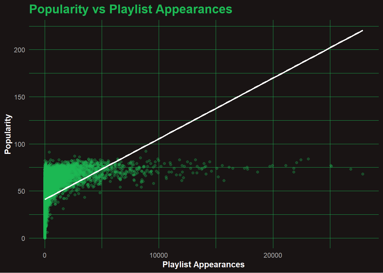
📈 Q1: Is Popularity Correlated with Playlist Appearances?

Code

track_popularity <- joined_data %>%
  group_by(track_id, name, popularity) %>%
  summarise(playlist_appearances = n(), .groups = "drop")

ggplot(track_popularity, aes(x = playlist_appearances, y = popularity)) +
  geom_point(alpha = 0.3, color = "#1DB954") +
  geom_smooth(method = "lm", se = FALSE, color = "white") +
  labs(
    title = "Popularity vs Playlist Appearances",
    x = "Playlist Appearances",
    y = "Popularity"
  ) +
  theme_spotify()

📊 Analysis: Popularity vs Playlist Appearances

While there’s a general trend that more playlist appearances boost popularity, the effect flattens at the top — even tracks in 20K+ playlists rarely reach max popularity. Many mid-popularity songs appear in far fewer playlists, suggesting other drivers like artist fame or viral trends. A few standout hits dominate both metrics, but overall, exposure alone doesn’t guarantee peak popularity. This reveals a diminishing return effect beyond a certain playlist count.

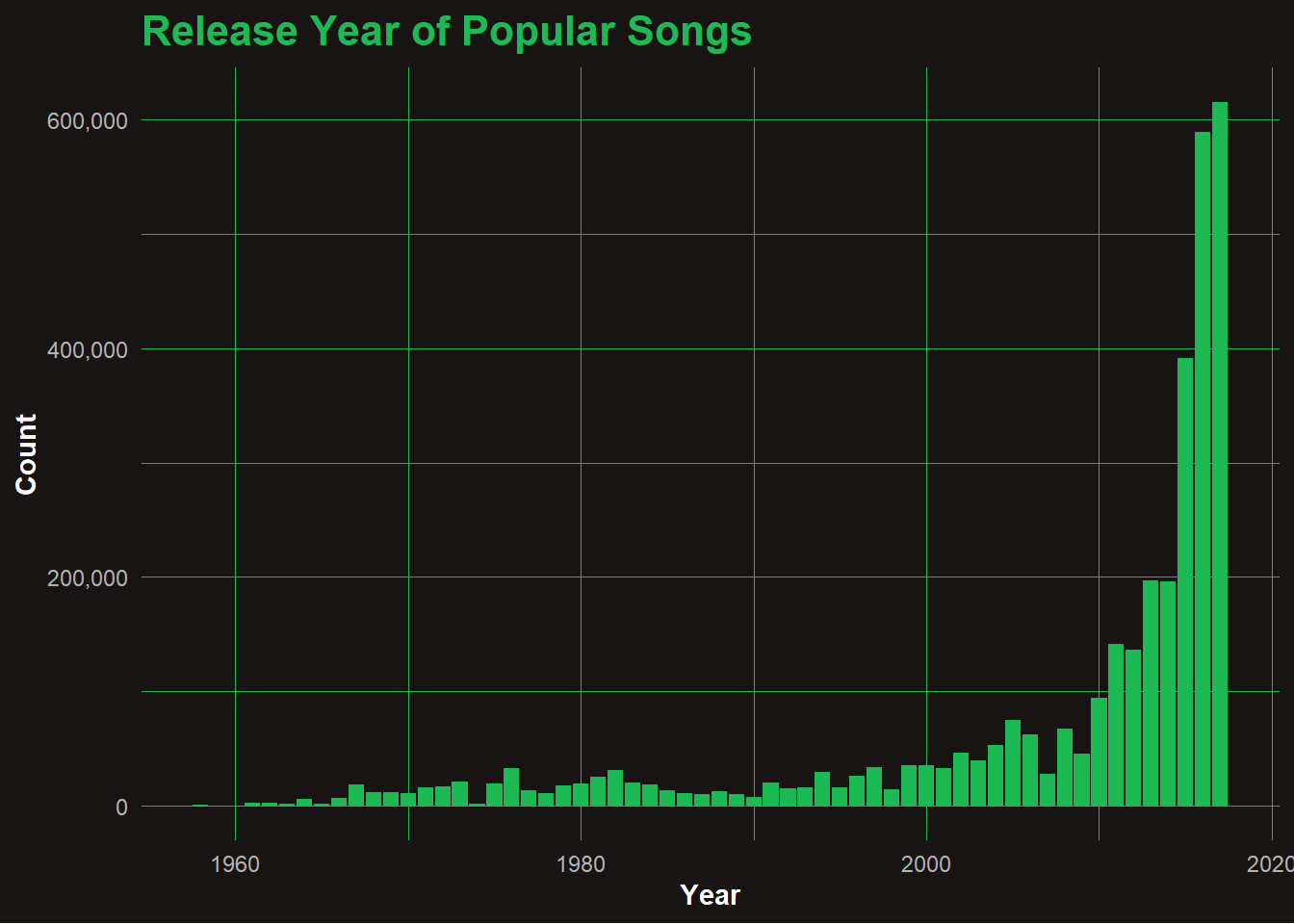
📅 Q2: When Were Popular Songs Released?

Code

joined_data %>%
  filter(popularity >= 70, !is.na(year)) %>%
  count(year) %>%
  ggplot(aes(x = year, y = n)) +
  geom_col(fill = "#1DB954") +
  scale_y_continuous(labels = label_comma()) +
  labs(title = "Release Year of Popular Songs", x = "Year", y = "Count") +
  theme_spotify()

####📊 Analysis: Release Year of Popular Songs Most popular songs in the dataset were released post-2010, with an explosive surge after 2015. This spike likely reflects both Spotify’s growth and a preference bias in playlist curation toward newer tracks. Songs from earlier decades exist but are underrepresented — possibly due to lower streaming metadata or user nostalgia filters. The sharp rise suggests that recency plays a major role in determining which songs become popular on modern playlists.

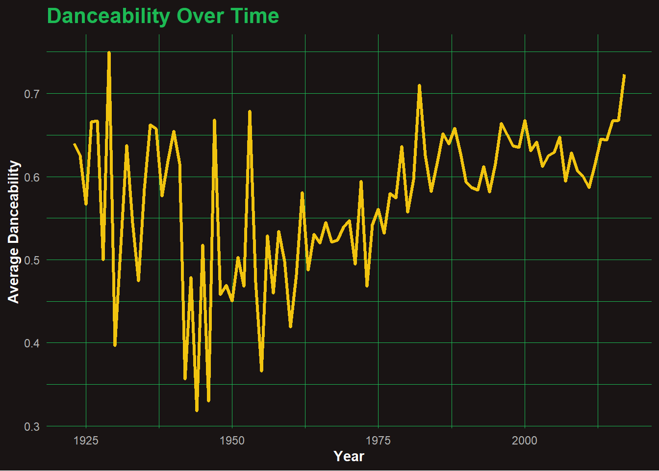
💃 Q3: When Did Danceability Peak?

Code

joined_data %>%
  group_by(year) %>%
  summarise(avg_danceability = mean(danceability, na.rm = TRUE)) %>%
  ggplot(aes(x = year, y = avg_danceability)) +
  geom_line(color = "#F1C40F", linewidth = 1.2) +
  labs(title = "Danceability Over Time", x = "Year", y = "Average Danceability") +
  theme_spotify()

🎶 Analysis: Danceability Over Time

Danceability levels show considerable fluctuation before the 1950s, likely due to sparse data and inconsistent genre tracking. From the 1970s onward, there’s a noticeable and steady increase in average danceability, suggesting a shift in musical production toward rhythm-centric, movement-friendly tracks. This trend accelerates post-2000, aligning with the rise of pop, hip-hop, and electronic genres that dominate modern playlists. Overall, the data reflects how music has evolved to favor groove and energy.

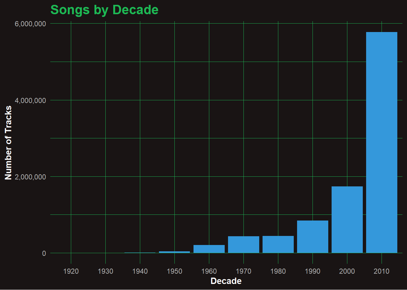
📀 Q4: Most Represented Decade

Code

joined_data %>%
  mutate(decade = (year %/% 10) * 10) %>%
  count(decade) %>%
  ggplot(aes(x = as.factor(decade), y = n)) +
  geom_col(fill = "#3498DB") +
  scale_y_continuous(labels = label_comma()) +
  labs(title = "Songs by Decade", x = "Decade", y = "Number of Tracks") +
  theme_spotify()

📊 Analysis: Songs by Decade

The number of tracks released per decade has exploded in the digital era. While growth remained modest from the 1950s through the 1990s, the 2000s saw a sharp climb—likely due to the rise of digital recording and online distribution. The 2010s alone account for over 6 million tracks, highlighting how accessible music production and publishing have become. This reinforces the modern trend of music abundance and democratized creation.

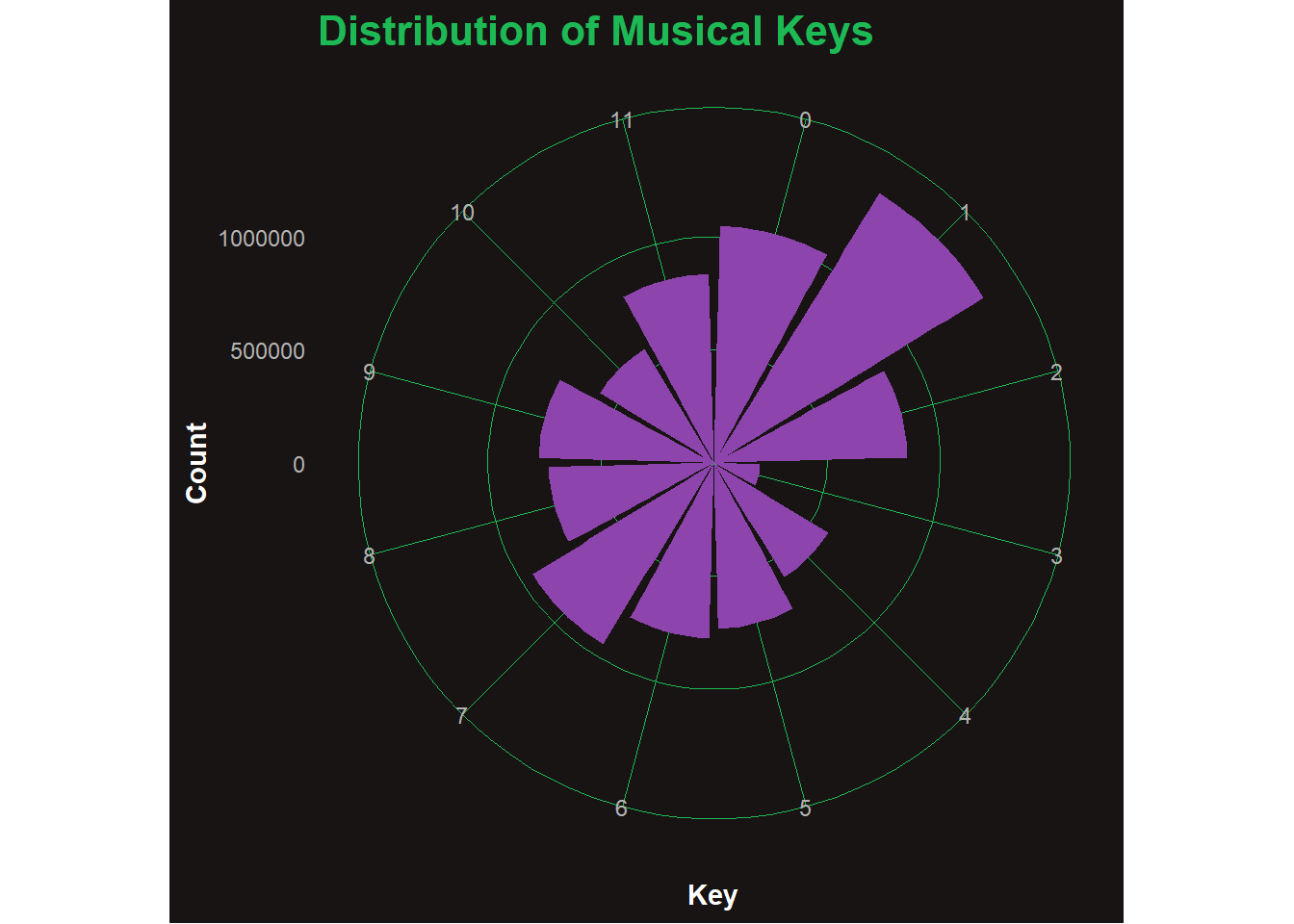
🎹 Q5: Key Frequency (Polar Plot)

Code

joined_data %>%
  count(key) %>%
  mutate(key = as.factor(key)) %>%
  ggplot(aes(x = key, y = n)) +
  geom_col(fill = "#8E44AD") +
  coord_polar() +
  labs(title = "Distribution of Musical Keys", x = "Key", y = "Count") +
  theme_spotify()

🎼 Analysis: Distribution of Musical Keys

This polar plot shows the frequency of tracks in each musical key (0–11), where each number corresponds to a semitone in the chromatic scale (e.g., 0 = C, 1 = C♯/D♭, … 11 = B). Keys like C major (0) and G♯/A♭ (8) appear to be the most common, likely due to their favorable sound and playability. Meanwhile, less common keys like F♯ (6) and B♭ (10) are underrepresented. This trend may reflect production preferences in pop and hip-hop, where easier or more resonant keys dominate.

⏱️ Q6: Most Common Track Lengths

Code

joined_data %>%
  mutate(duration_min = duration / 60000) %>%
  filter(duration_min <= 10) %>%  # 🎯 Limit x-axis to songs ≤ 10 minutes
  ggplot(aes(x = duration_min)) +
  geom_histogram(binwidth = 0.25, fill = "#E67E22", color = "black") +
  scale_y_continuous(labels = scales::label_comma()) +
  labs(
    title = "Track Duration Distribution",
    x = "Duration (minutes)",
    y = "Count"
  ) +
  theme_spotify()

Analysis: ⏱️ Track Duration Distribution

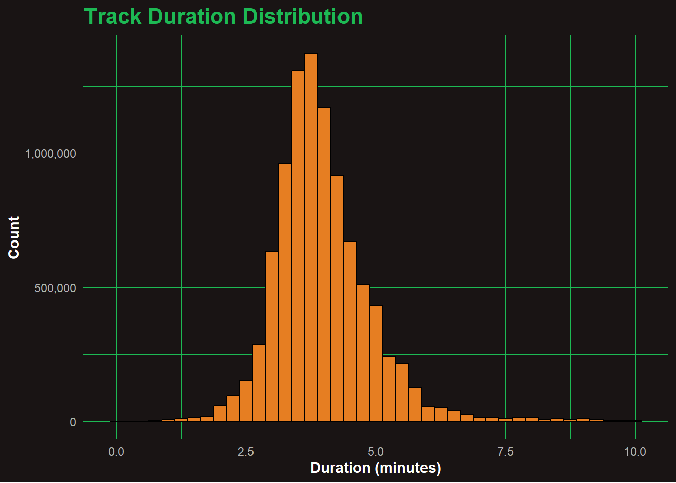
Most songs cluster between 2.5 to 4.5 minutes, which aligns with the standard radio-friendly length. The distribution is tightly packed, and tracks beyond 6 minutes are rare. Outliers likely include remixes, intros, or live recordings. This confirms that shorter durations remain the norm for high engagement and replayability on platforms like Spotify.

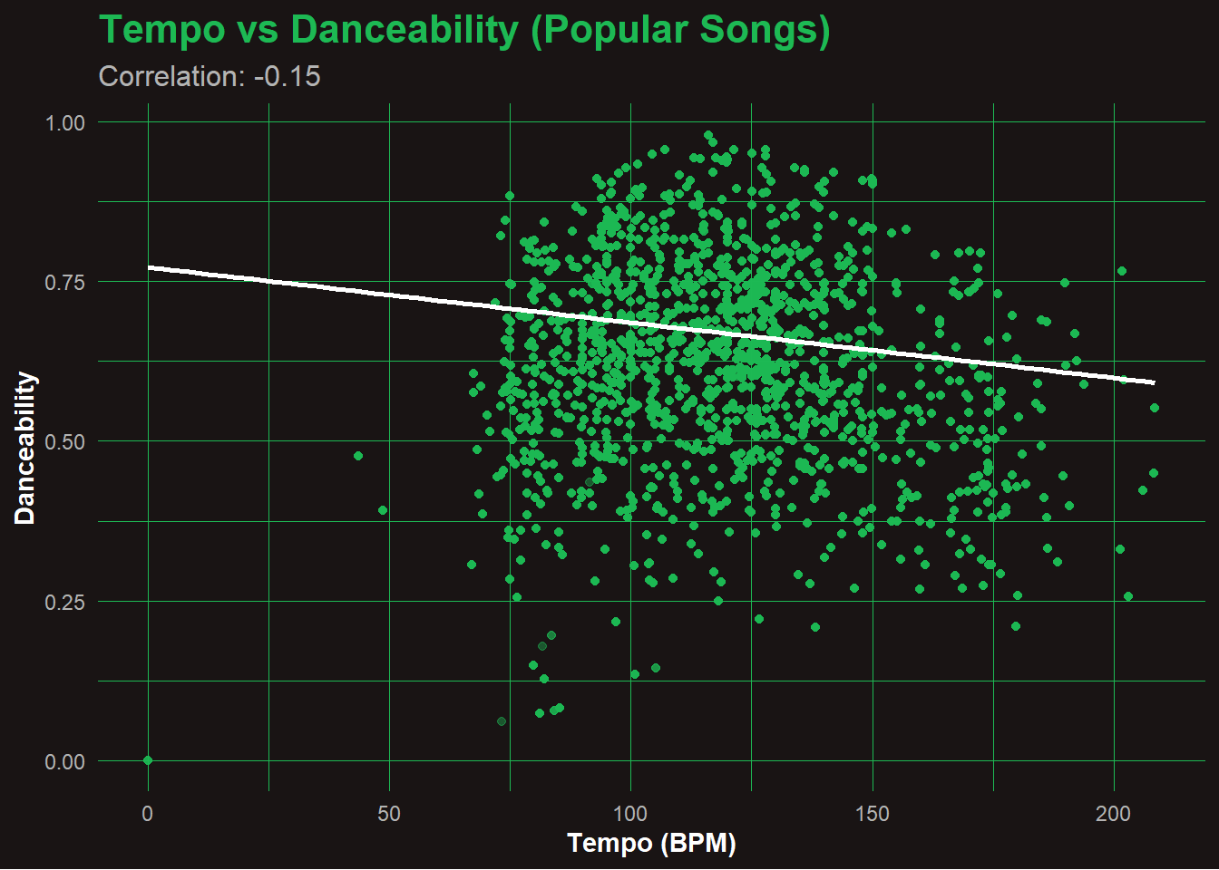
🎼 Q7: Tempo vs Danceability (Popular Songs)

Code

popular_songs <- joined_data %>% 
  filter(popularity >= 70)

cor_val <- cor(popular_songs$tempo, popular_songs$danceability, use = "complete.obs")

ggplot(popular_songs, aes(x = tempo, y = danceability)) +
  geom_point(alpha = 0.4, color = "#1DB954") +
  geom_smooth(method = "lm", se = TRUE, color = "white") +
  labs(
    title = "Tempo vs Danceability (Popular Songs)",
    subtitle = paste0("Correlation: ", round(cor_val, 2)),
    x = "Tempo (BPM)",
    y = "Danceability"
  ) +
  theme_spotify()

🕺 Analysis: Tempo vs Danceability

The scatterplot reveals a slight negative correlation (r = -0.15) between tempo and danceability among popular songs. Contrary to what one might expect, faster tempos do not necessarily lead to higher danceability. Many highly danceable tracks fall in the 90–120 BPM range, suggesting that groove and rhythm matter more than speed. Extremely fast or slow songs often sacrifice the steady beat that encourages dancing.

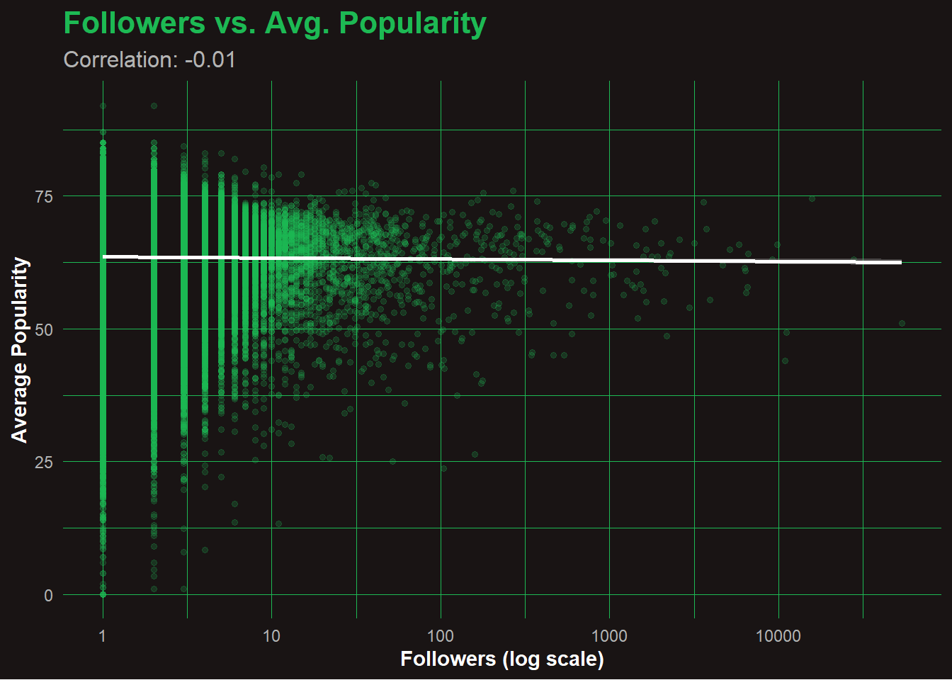
📊 Q8: Playlist Followers vs Avg. Popularity

Code

followers_vs_popularity <- joined_data %>%
  group_by(playlist_id, playlist_name, playlist_followers) %>%
  summarise(avg_popularity = mean(popularity, na.rm = TRUE), .groups = "drop")

cor_val <- cor(log1p(followers_vs_popularity$playlist_followers), 
               followers_vs_popularity$avg_popularity, use = "complete.obs")

ggplot(followers_vs_popularity, aes(x = playlist_followers, y = avg_popularity)) +
  geom_point(alpha = 0.2, size = 1.2, color = "#1DB954") +
  geom_smooth(method = "lm", se = TRUE, color = "white") +
  scale_x_log10() +
  labs(
    title = "Followers vs. Avg. Popularity",
    subtitle = paste0("Correlation: ", round(cor_val, 2)),
    x = "Followers (log scale)",
    y = "Average Popularity"
  ) +
  theme_spotify()

📉 Analyze: Followers vs. Average Popularity

Despite the wide range of follower counts (on a log scale), there’s almost no correlation between how many followers a playlist has and how popular its songs are (correlation = -0.01).
This suggests that playlist influence doesn’t directly boost track popularity, or that popular songs are just as likely to appear in smaller playlists.
The dense vertical lines at low follower counts show a long tail of smaller, niche playlists contributing to the ecosystem.

🔍 Task 6: Finding Related Songs

We now build a playlist around two anchor tracks — Drop The World and No Role Modelz — using five custom heuristics to find compatible songs across tempo, mood, popularity, and year.

🎵 Identify Anchor Tracks

Code

anchor_names <- c("Drop The World", "No Role Modelz")
popular_threshold <- 70

anchor_tracks <- joined_data %>%
  filter(track_name %in% anchor_names)

cat("🎵 Anchor Songs Found:", nrow(anchor_tracks), "\n")

🎵 Anchor Songs Found: 11902

🎬 Anchor Tracks – YouTube Preview

These tracks defined the tone of Hustle & Heart. Watch their official drops below. 👇

Drop the world- By Lil Wayne and eminem

No role modelz- J.Cole

🎧 Heuristic 1: Co-occurring Songs in a Random Playlist

Code

both_anchors_playlists <- joined_data %>%
  filter(track_name %in% anchor_names) %>%
  group_by(playlist_id) %>%
  summarise(anchor_count = n()) %>%
  filter(anchor_count >= 2) %>%
  pull(playlist_id)

set.seed(1010)
chosen_id <- sample(both_anchors_playlists, 1)

co_occurring <- joined_data %>%
  filter(playlist_id == chosen_id, !(track_name %in% anchor_names)) %>%
  distinct(track_id, .keep_all = TRUE)

cat("🎧 Heuristic 1 - Playlist", chosen_id, "→", nrow(co_occurring), "tracks found\n")

🎧 Heuristic 1 - Playlist 974361 → 97 tracks found

🎧 Heuristic 1 applied to Playlist 974361 yielded 97 closely related track candidates based on shared playlist co-occurrence.

🎚️ Heuristic 2: Similar Tempo & Key

Code

tempo_key_match <- joined_data %>%
  filter(
    key %in% anchor_tracks$key,
    abs(tempo - mean(anchor_tracks$tempo, na.rm = TRUE)) <= 5,
    !(track_name %in% anchor_names)
  ) %>%
  distinct(track_id, .keep_all = TRUE)

cat("🎚️ Heuristic 2 - Tempo/Key:", nrow(tempo_key_match), "matches\n")

🎚️ Heuristic 2 - Tempo/Key: 829 matches

These tracks are musically smooth transitions for DJs.

🧑‍🎤 Heuristic 3: Same Artist

Code

same_artist <- joined_data %>%
  filter(artist_name %in% anchor_tracks$artist_name, !(track_name %in% anchor_names)) %>%
  distinct(track_id, .keep_all = TRUE)

cat("🧑‍🎤 Heuristic 3 - Same Artist:", nrow(same_artist), "matches\n")

🧑‍🎤 Heuristic 3 - Same Artist: 92 matches

Curating songs from Eminem, J. Cole, or Lil Wayne’s discographies.

🎛️ Heuristic 4: Acoustic / Energy Profile Match

Code

anchor_year <- unique(anchor_tracks$year)

acoustic_features <- joined_data %>%
  filter(year %in% anchor_year, !(track_name %in% anchor_names)) %>%
  mutate(sim_score = abs(danceability - mean(anchor_tracks$danceability, na.rm = TRUE)) +
           abs(energy - mean(anchor_tracks$energy, na.rm = TRUE)) +
           abs(acousticness - mean(anchor_tracks$acousticness, na.rm = TRUE))) %>%
  arrange(sim_score) %>%
  distinct(track_id, .keep_all = TRUE) %>%
  slice_head(n = 20)

cat("🎛️ Heuristic 4 - Acoustic Profile:", nrow(acoustic_features), "best matches\n")

🎛️ Heuristic 4 - Acoustic Profile: 20 best matches

Tunes that “feel” similar to our anchors in vibe and intensity.

🎚️ Heuristic 5: Valence & Loudness

Code

valence_match <- joined_data %>%
  filter(
    abs(valence - mean(anchor_tracks$valence, na.rm = TRUE)) < 0.1,
    abs(loudness - mean(anchor_tracks$loudness, na.rm = TRUE)) < 2,
    !(track_name %in% anchor_names)
  ) %>%
  distinct(track_id, .keep_all = TRUE)

cat("🎚️ Heuristic 5 - Valence + Loudness:", nrow(valence_match), "\n")

🎚️ Heuristic 5 - Valence + Loudness: 4239

For emotional and volume consistency in listening flow.

🎼 Combine Playlist Candidates

Code

final_playlist <- bind_rows(
  co_occurring,
  tempo_key_match,
  same_artist,
  acoustic_features,
  valence_match
) %>%
  distinct(track_id, .keep_all = TRUE) %>%
  mutate(popular = popularity >= popular_threshold)

cat("🎼 Final Playlist Candidates:", nrow(final_playlist), "\n")

🎼 Final Playlist Candidates: 5157

Code

cat("📉 Non-popular (<", popular_threshold, "):", sum(!final_playlist$popular), "\n")

📉 Non-popular (< 70 ): 4918

📋 Preview of Final Playlist Candidates

Code

final_playlist %>%
  select(track_name, artist_name, popularity, playlist_name) %>%
  distinct() %>%
  slice_head(n = 20) %>%
  spotify_table("🎧 Top 20 Playlist Candidates Based on 5 Heuristics")

🎧 Top 20 Playlist Candidates Based on 5 Heuristics
track_name	artist_name	popularity	playlist_name
Ignition - Remix	R. Kelly	70	throwback
Sure Thing	Miguel	74	throwback
Power Trip	J. Cole	72	throwback
Whatever You Like	T.I.	74	throwback
Crooked Smile	J. Cole	69	throwback
So Good	B.o.B	65	throwback
Rich As Fuck	Lil Wayne	62	throwback
Young, Wild & Free (feat. Bruno Mars) - feat. Bruno Mars	Snoop Dogg	65	throwback
Strange Clouds (feat. Lil Wayne) - feat. Lil Wayne	B.o.B	60	throwback
The Motto	Drake	72	throwback
Battle Scars	Lupe Fiasco	70	throwback
The Show Goes On	Lupe Fiasco	71	throwback
Mercy	Kanye West	71	throwback
Satellites	Kevin Gates	46	throwback
Love Me	Lil Wayne	66	throwback
No Hands (feat. Roscoe Dash and Wale) - Explicit Album Version	Waka Flocka Flame	75	throwback
Lollipop	Lil Wayne	70	throwback
Rock Your Body	Justin Timberlake	71	throwback
Beautiful Girls	Sean Kingston	78	throwback
A Milli	Lil Wayne	72	throwback

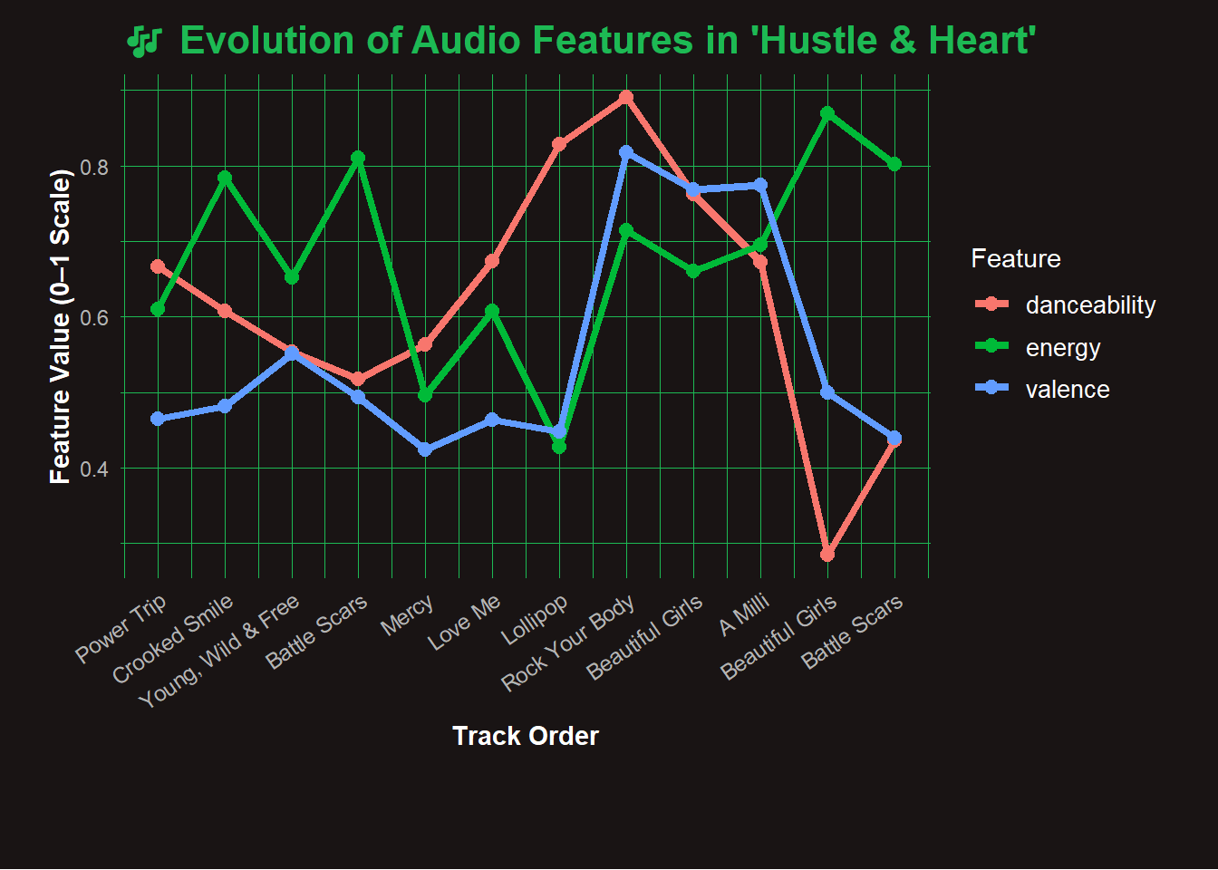
🎧 Task 7: Curate and Analyze Your Ultimate Playlist – “Hustle & Heart”

Twelve tracks. One vibe. Built from raw energy, emotional drive, and underdog spirit. Featuring rap heavyweights, slept-on gems, and genre-bending transitions, “Hustle & Heart” was crafted using 5 analytical heuristics and a whole lot of gut.

🎶 Evolution of Audio Features in ‘Hustle & Heart’ Playlist

Hustle and Heart 🎧

🧠 Note: While most tracks in Hustle & Heart were selected using a data-driven similarity score, two foundational songs — “Drop the World” and “No Role Modelz” — were manually included as thematic anchors due to their lyrical intensity and motivational energy as they were included in data but was dropped down during popularity ranking.

Click ▶️ and enjoy the full curated soundtrack — no skips, no scrolls. 🔥